Three new models have been added to the AutoEZ samples folder as of maintenance
release v. 2.0.6.
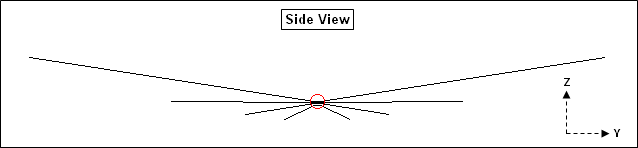
With model "Fan Dipole Splayed Elements.weq" you can set variables to easily
configure the wires like this, for example, which might represent a fan strung
between two supports with a "catenary sag" in the center.
http://ac6la.com/adhoc/fanocf1.png
Change the variables another way to get this kind of configuration, inverted
vees held up by a center support and two shorter end supports.
http://ac6la.com/adhoc/fanocf2.png
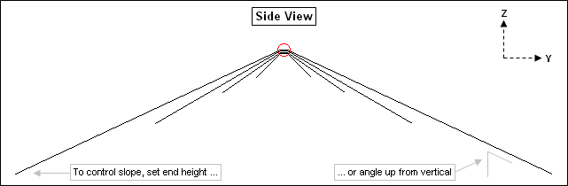
To control the slope (if any) for each side of each element you can set either
the height of the outer end or the angle of the wire up from vertical.
Whichever you enter will be used along with the total wire length and center
height to generate the correct coordinates in the wires table. In addition,
the corresponding "other" value (angle or end height) will be shown. The two
sides need not have the same slope.
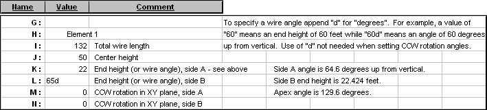
Here is an extract from the Variables sheet tab showing how you control the
first (top) element. Other groups of variables, not shown, control the other
elements. The number of elements in the model is adjustable from 1 to 6. (Set
the number of elements first, then set other groups of variables as
appropriate.)
http://ac6la.com/adhoc/fanocf3.png
If you would prefer to work with meters or inches instead of feet use the
"Change Units" button (with the "retain formulas" option) and then reset the
variable values as desired.
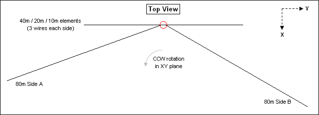
You can also rotate the outer ends of one or more elements in the XY plane,
perhaps to increase the separation between wires or take advantage of available
supports. Here is a top-down view of a set of inverted vees with the outer
ends of the 80m element rotated in a somewhat arbitrary manner, just for
illustration. Side A of the 80m element has been rotated 20° CCW in the XY
plane and side B has been rotated 330° (or -30°) CCW.
http://ac6la.com/adhoc/fanocf4.png
As you change variables be sure to frequently use the "View Ant" button to
verify that the wires of the model are positioned as you intended. Make sure
that no wires cross on top of other wires. Also be careful to not enter
"impossible" combinations. For example, if an element is 32 ft long (16 ft
each side) with a center height of 50 ft, and you set an end height at 20 ft
(impossible), you'll see an Excel error code of "#NUM!" for the slope angle.
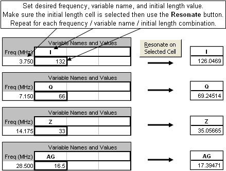
Once you have the model configured as desired the next step is to fine-tune the
element lengths to be resonant at your chosen set of frequencies. On the
Calculate sheet enter a frequency, the variable name that controls the total
length of the corresponding element, and a starting length value. With the
length cell selected click the "Resonate" button. Repeat this process for
other frequencies, variable names, and lengths.
http://ac6la.com/adhoc/fanocf5.png
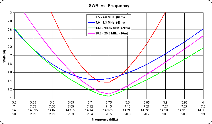
You may then wish to run a frequency sweep across multiple bands to see the SWR
patterns. Remember that you are free to do other things such as check email or
surf the web while the calculations are running. Assuming you calculated
multiple bands at the same time, you can use the "Set/Lock Scales" button on
the Custom chart sheet tab to "zoom in" on a particular frequency range of
interest (discussed more later). This composite chart illustrates the effect.
http://ac6la.com/adhoc/fanocf6.png
############
With model "Fan Dipole Parallel Elements.weq" you can easily create a
configuration in which the wires are separated by a fixed spacing, typically a
few inches to a few feet. This animated gif illustrates that the separation
between elements, controlled by a variable, stays constant as the slope angle
of the elements is changed.
http://ac6la.com/adhoc/fanocf7ani.gif
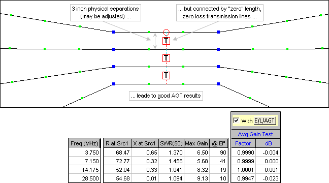
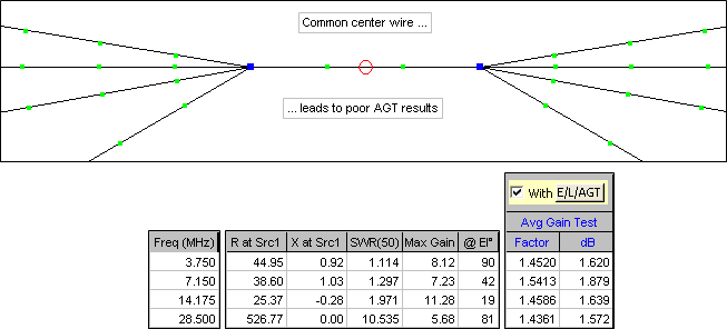
In both the "Splayed" and "Parallel" fan models the elements are *physically*
separated by a small amount at the centers but are *electrically* joined by
"zero" length (almost) and zero loss NEC transmission lines. This technique
was described by L.B. Cebik, W4RNL (SK), see reference below. Making the
connection between elements this way, as opposed to building a model with the
elements physically connected to a common center wire, results in much better
Average Gain Test results, hence more reliable impedance and gain values. As
an example, using an exploded view of the splayed element model shown earlier:
http://ac6la.com/adhoc/fanocf8.png
Now compare the above Average Gain Test results with those shown below.
http://ac6la.com/adhoc/fanocf9.png
Even after correcting the source resistance and gain by the AGT values, when
using a common center wire the results are still unreliable at the higher
frequencies.
############
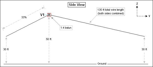
With model "OCF Dipole.weq" you can use variables to set the total wire length
and the percent from end for the feedpoint position. As with the fan models
you can control the slope angle of both the short and long sections by
specifying either end heights or wire angles. An additional variable lets you
change the impedance ratio of the balun at the feedpoint, such as 1:4 or 1:6.
Here is an example of a typical layout.
http://ac6la.com/adhoc/fanocf10.png
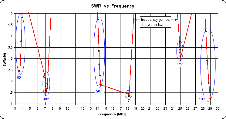
And here is the SWR response for this particular configuration. Six
frequencies were used for each of 8 bands, 80/40/30/20/17/15/12/10 meters.
Using the same number of frequencies for each band means that you can take
advantage of the "Subsets" button on the Custom chart tab to see the response
for each band separately (discussed more later), although the illustration
below shows all bands together. In this example the max SWR was clipped at 5:1
for plotting so some bands don't show all 6 frequency dots and other bands
don't show any dots at all. The straight trace lines connecting groups of dots
are merely the "frequency jumps" from one band to the next and can be ignored.
http://ac6la.com/adhoc/fanocf11.png
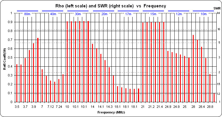
An alternate method to plot SWR is to use "EZNEC spacing" for the Y axis of the
chart, which means a reflection coefficient chart with SWR gridlines. (EZNEC
SWR charts show only the SWR values but the vertical spacing is per the
corresponding reflection coefficient value.) In addition, for the X axis of
the chart you can choose "Frequency - Column" rather than "Frequency - Line".
That eliminates the extraneous straight line traces between the bands. So in
the chart below, each band is shown as 6 columns rather than six dots connected
by lines. The reflection coefficient (rho) values are on the left vertical
scale, the corresponding SWR values are on the right.
http://ac6la.com/adhoc/fanocf12.png
############
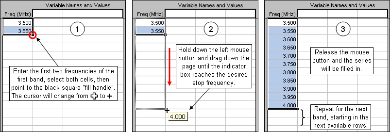
When dealing with multiband antennas there is always the question of which
frequencies to calculate. Of course you can use something like Start 3.0, Stop
30.0, Step 0.05 MHz but that results in many frequencies of little interest
unless you are trying to get a feel for the relationship between SWR dips. An
alternative is to calculate groups of frequencies for each band, skipping the
frequencies between bands. The Excel "fill handle" makes it easy to enter such
groups, as illustrated below.
http://ac6la.com/adhoc/fanocf13.png
The number of frequencies for each band is determined by the delta between the
first two entries for each band. You can use the same step size, say 0.05 or
0.025 MHz for each band, or you can divide each band into the same number of
steps. For example (using ITU Region 2 band plans), you might enter 3, 3.55,
... 4 to get 11 frequencies for 80m, then 7, 7.03, ... 7.3 to get 11
frequencies for 40m, and so on.
When you save the model the current set of frequencies on the Calculate sheet
will be saved as well so there will be no need to repeat the entry process the
next time you open the model.
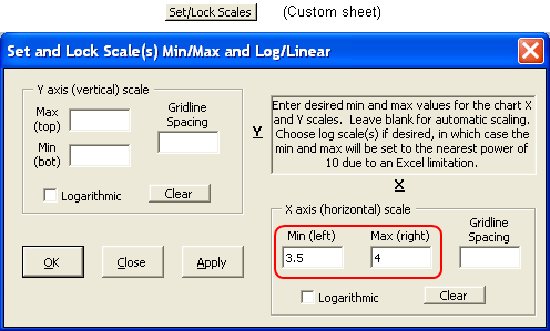
After you have calculated several groups of frequencies (that is, several
bands) there are two methods available to plot a single band rather than all
bands. You can use the "Set/Lock Scales" button on the Custom chart sheet tab,
setting the min and max of the X axis (typically Frequency) as desired. For
example, to plot just the 80m band you could enter min and max values like this.
http://ac6la.com/adhoc/fanocf14.png
If you click the "Apply" button the dialog window will stay open so you can
easily change to a different min/max (different band). If you click "OK" the
dialog window will close.
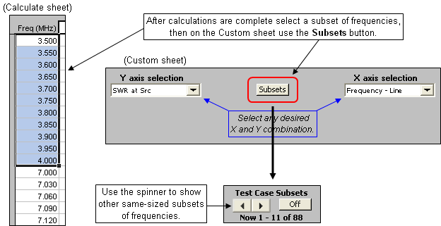
There is an alternate way to show separate bands on the Custom chart if you
have calculated the same number of frequencies for each band. After all
calculations are complete, on the Calculate sheet select (drag through,
highlight) just that subset of frequencies that were used for the first band.
Then on the Custom sheet click the "Subsets" button.
http://ac6la.com/adhoc/fanocf15.png
The "Subsets" button will be replaced with a spinner button. You can use that
spinner to advance to other bands, that is, other subsets of frequencies.
############
References:
Cebik article on using "zero" length transmission lines to connect fan elements:
http://www.antennex.com/w4rnl/col0507/amod111.html
Stanford Research Institute paper on fan dipoles:
http://www.rebelwolf.com/HFD.pdf
Construction ideas and other tips for fan dipoles:
http://www.hamuniverse.com/multidipole.html
http://www.hamuniverse.com/ae5jumultibanddipole.html
http://www.hamuniverse.com/w6hdgfandipole.html
http://www.hamuniverse.com/kj4iif1608040fandipole.html
http://ve2xip.cactus.net/?p=1342
Cebik articles on OCF dipoles:
http://w4rnl.net46.net/gup9.html
http://w4rnl.net46.net/gup10.html
http://w4rnl.net46.net/gup11.html
http://w4rnl.net46.net/download/iocf.pdf
http://w4rnl.net46.net/download/tlocf.pdf
Construction ideas and other tips for OCF dipoles:
http://www.w8ji.com/windom_off_center_fed.htm
http://hamwaves.com/cl-ocfd/index.html
http://www.buxcomm.com/windom.htm
http://www.balundesigns.com/OCF%20Antenna.pdf
http://www.designerweb.net/downloads/OCF-dipoles.pdf
The "OCF Dipole.weq" model allows a second element to be included. This
article explains why you might want to do that:
http://dev.n8it.org/acs/documents/off%20center%20fed%20dipole.pdf
Quick and simple review of sine, cosine, and tangent trig functions, in case
you are curious about all the Excel formulas used in the models:
http://www.mathsisfun.com/algebra/sohcahtoa.html
############
For more information on AutoEZ and to download a free demo version see:
http://ac6la.com/autoez.html
With the demo you will not be able to do any calculations because of the large
number of segments in each model. However, you can change the variables as
desired, use the "View Ant" button to see what you have created, then switch
over to the EZNEC window and do calculations directly in EZNEC.
Current AutoEZ users: If you would like to update your copy of AutoEZ to the
latest level which includes the above models, download the most recent
installer ("autoezsetup.exe") program. The download link is shown in your
purchase confirmation email. If you have misplaced that email please contact
me directly for assistance.
Dan, AC6LA
_______________________________________________
_______________________________________________
TowerTalk mailing list
TowerTalk@contesting.com
http://lists.contesting.com/mailman/listinfo/towertalk
|